4. Performance

4.1. Measuring performance

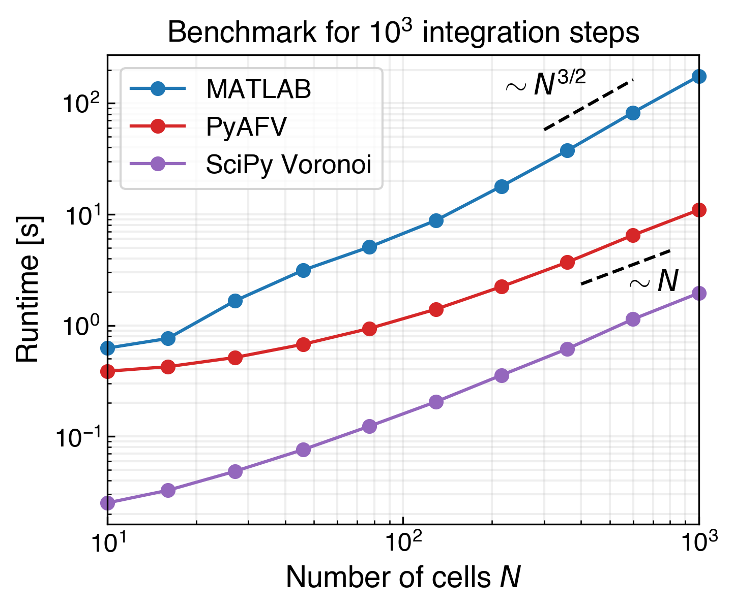
PyAFV has been benchmarked against the MATLAB implementation of the active finite Voronoi model from Ref. [1] by measuring the wall-clock runtime for simulations of varying system sizes. The results are shown in the figure; each data point corresponds to \(10^3\) integration steps, averaged over three independent runs. The results show that PyAFV exhibits near-linear scaling, approximately \(\mathcal{O}(N)\)—comparable to the scaling behavior of SciPy’s Voronoi implementation scipy.spatial.Voronoi—whereas the original MATLAB code scales more steeply, at roughly \(\mathcal{O}(N^{3/2})\). This difference will lead to a significant speedup, particularly for large systems (\(N\gtrsim 10^3\)).

Note

All benchmark results were obtained on a MacBook Pro (14-in, 2024) equipped with an Apple M4 Pro chip (12-core) and 24 GB of RAM, running macOS 15.6. The MATLAB implementation was executed using MATLAB R2025a, while PyAFV was run using Python 3.13.5 with the PyAFV v0.4.3 default Cython backend (PyAFV v0.4.12 for parallel build benchmark).

4.2. Benchmarking backends

In addition, there is a set of lightweight benchmarks in tests using pytest-benchmark, e.g., test_bench_build.py compares the runtimes of the Cython and pure-Python backends . To run it:

(.venv) $ uv run pytest tests/test_bench_build.py --benchmark-only --benchmark-warmup on --benchmark-histogram

This will display the benchmark results and generate an interactive SVG histogram file (click to see the detailed timing results for each method):

The histogram above summarizes the runtimes of the core routines invoked by pyafv.FiniteVoronoiSimulator.build() for a system of \(N=1000\) cells. The test_scipy_voronoi benchmark measures the execution time of SciPy’s Voronoi tessellation, which serves as a baseline for comparison. This SciPy routine is called internally by pyafv.FiniteVoronoiSimulator._build_voronoi_with_extensions(), corresponding to the test_build_voronoi benchmark shown in the histogram. From this comparison, we see that SciPy’s Voronoi computation accounts for approximately 60% of the total runtime of that method.

Hint

The suffixes [accel] and [fallback] in the benchmark names indicate whether the Cython backend or the pure-Python fallback implementation was used.

The remaining dominant cost arises from the additional per-cell processing performed in pyafv.FiniteVoronoiSimulator._per_cell_geometry(). As shown in the histogram, the Cython-backed implementation substantially reduces the runtime of this step, bringing it down to a level comparable to that of SciPy’s Voronoi tessellation.

4.3. Benchmarking parallel build

Build-time benchmark for pyafv.FiniteVoronoiSimulator and pyafv.ParallelFiniteVoronoiSimulator.

This figure shows the cost of a single pyafv.FiniteVoronoiSimulator.build() call with connect=False against the domain-decomposed multiprocess implementation. For each system size, the same ten randomly generated point sets were used for all methods; the bars show the mean build time, while the right panel shows the speedup relative to pyafv.FiniteVoronoiSimulator. Parallel timings were measured with a persistent worker pool and three unmeasured warm-up builds, so the reported times do not include one-time worker startup. The number of workers is set equal to the number of domains.

For very small systems, multiprocessing overhead dominates. In this benchmark, the parallel implementation is slower than the single-process simulator at \(N=100\), but becomes faster by \(N=1000\). For larger systems, local domain decomposition gives substantial speedups: the 4 x 3 setup reaches about \(4.9\times\) at \(N=10^4\), \(6.8\times\) at \(N=10^5\), and \(6.9\times\) at \(N=10^6\). The speedup is not perfectly linear in the number of workers, likely because the benchmark was run on a laptop with 8 performance cores and 4 efficiency cores rather than on a uniform multi-core CPU.

The following figures show benchmark runs on the Rockfish HPC cluster at Johns Hopkins University. The first figure corresponds to runs on the shared partition (32 cores/node), while the second shows results from the parallel partition (48 cores/node). The serial pyafv.FiniteVoronoiSimulator benchmark was allocated 16 GB of memory to avoid out-of-memory (OOM) failures; on Rockfish, this allocation corresponded to 5 CPUs on both partitions. For the parallel simulator runs, both the number of allocated CPUs and the number of workers were set equal to the number of domains. Compared with the laptop benchmark, the parallel speedup scales more cleanly with the number of workers.

JHU Rockfish shared partition build-time benchmark.

JHU Rockfish parallel partition build-time benchmark.

The optimal decomposition depends on the number of points and the CPU resources available on the machine. In this benchmark, using more domains generally helps over the tested range, but the best choice should still be checked for each workload because worker scheduling, inter-process data transfer, result merging, and CPU affinity all depend on the hardware and launch configuration.

4.4. Benchmarking hybrid parallel build: MPI + Python multiprocessing

Benchmark for a hybrid Python multiprocessing + MPI wrapper on JHU Rockfish parallel partition.

The hybrid benchmark uses MPI for a coarse domain decomposition and pyafv.ParallelFiniteVoronoiSimulator inside each rank for a second local multiprocessing decomposition; see Multi-node parallelism: MPI. A label such as (2 x 2) x (4 x 3) means that the full system is first decomposed into a 2 x 2 MPI-rank grid, and each rank then decomposes its local point set into a 4 x 3 worker grid.

The hybrid timing includes the full wrapper step: coarse domain decomposition on rank 0, MPI broadcast of the domains, local multiprocessing builds, MPI gather of owned-cell forces, and force assembly on rank 0. For the hybrid benchmark runs, the number of Slurm tasks was set to the number of coarse MPI domains, and --cpus-per-task was set to the number of local multiprocessing subdomains. For example, the (2 x 2) x (4 x 3) case was launched with 4 MPI ranks and 12 CPUs (12 workers) per rank, for a total of 48 workers.

The equal-total-CPU comparisons are 8 x 6, (1 x 2) x (6 x 4), and (2 x 2) x (4 x 3), all of which use 48 CPUs (48 workers) in total. The hybrid versions are slightly faster for larger systems in this benchmark. This may be explained by the fact that the pure multiprocessing run has one parent process managing 48 workers, while the hybrid runs distribute that Python multiprocessing coordination across two or four MPI ranks. The hybrid benchmark also gathers and merges only owned-cell forces, while pyafv.ParallelFiniteVoronoiSimulator.build() returns a fuller diagnostic dictionary.

The (1 x 2) x (8 x 6) case is less efficient than might be expected from its 96 total workers, corresponding to 96 allocated CPUs. One likely reason is the launch layout: the parallel partition has 48 cores per node, so this configuration requires two nodes and therefore cross-node MPI communication. By contrast, the 48-worker (1 x 2) x (6 x 4) and (2 x 2) x (4 x 3) cases can fit on a single node, which reduces MPI communication overhead.