2. Examples
Note
To run the examples below, you need to install the tqdm package for progress bars. The Jupyter Notebooks in examples/jupyter/ additionally require jupyter and ipywidgets as well.
2.1. Relaxation to mechanical equilibrium
The following example shows how 100 cells relax to mechanical equilibrium from a squeezed initial configuration using the PyAFV package.
import numpy as np
import matplotlib.pyplot as plt
import tqdm
import pyafv as afv


np.random.seed(42)

N = 100         # number of cells
radius = 1.0    # maximal radius
mu = 1.0        # mobility
dt = 0.01       # time step

# Parameter set
phys = afv.PhysicalParams(
    r=radius,
    A0=np.pi*(radius**2),
    P0=4.8*radius,
    KA=1.0,
    KP=1.0,
    Lambda=0.2
)

# Do not set delta unless you know what you are doing.
# We set it to zero here for comparison with the our primitive results.
phys = phys.replace(delta=0.0)

# Initial positions
pts = np.random.rand(N, 2)*0.3 + 0.35  # shape (N,2)
pts *= 25.

# Initialize simulator
sim = afv.FiniteVoronoiSimulator(pts, phys)

# Plot initial configuration
fig, ax = plt.subplots()
sim.plot_2d(ax=ax)
plt.show()

# Relaxation to mechanical equilibrium
for _ in tqdm.tqdm(range(1000), desc="Relaxation"):
    diag = sim.build()
    forces = diag["forces"]
    pts += mu * forces * dt
    sim.update_positions(pts)

# Plot relaxed configuration
fig, ax = plt.subplots()
sim.plot_2d(ax=ax)
plt.show()
See the plotted figures below:
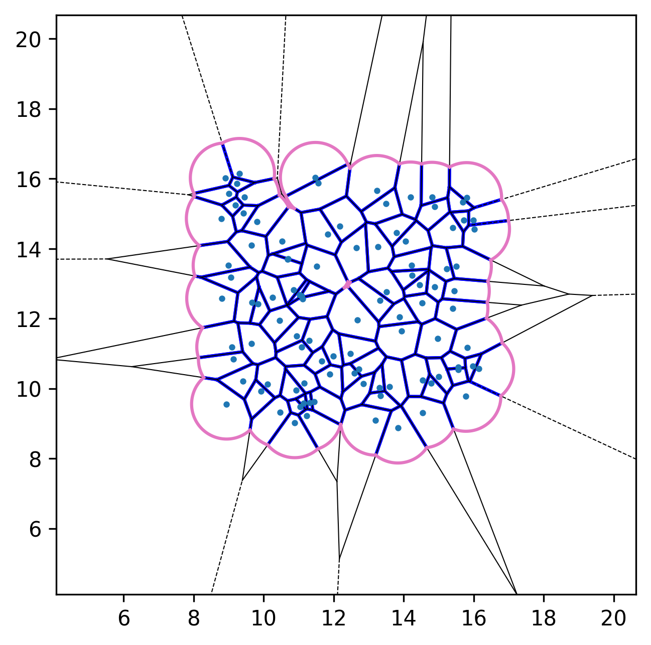
Initial configuration. |
After relaxation. |
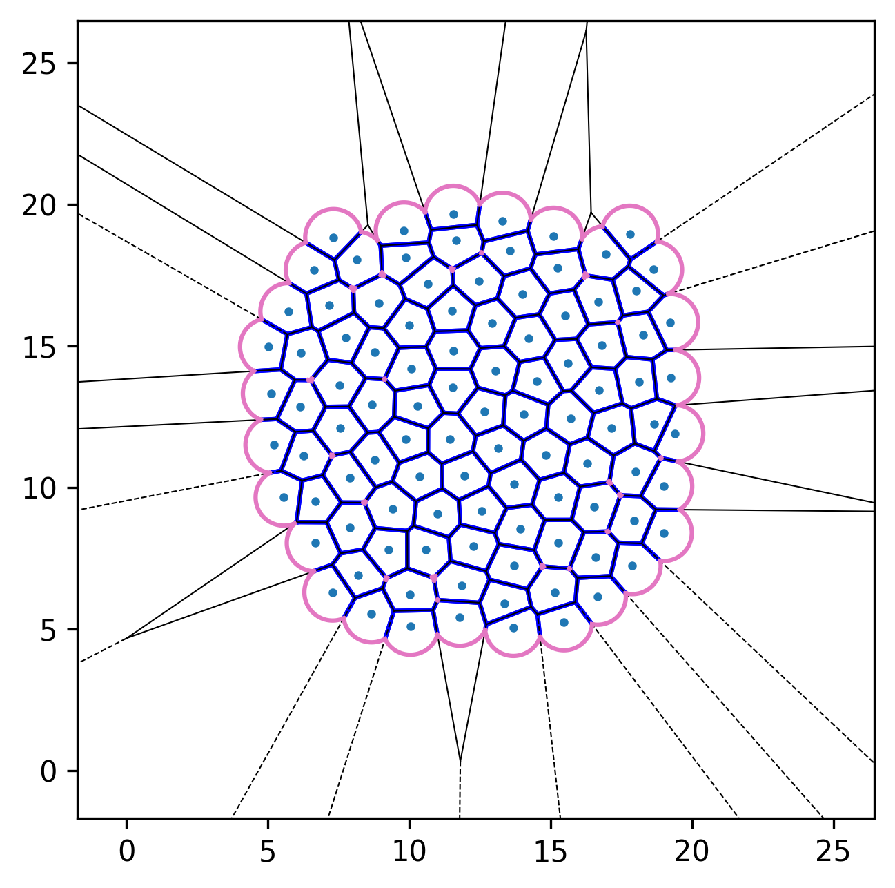
2.2. Active finite Voronoi (AFV) dynamics
We can incorporate self-propulsion (active-Brownian-like dynamics) for each cell to model active-matter systems. The resulting equation of motion is
where \(\mu\) is the mobility, the interaction force on cell \(\mathbf{F}_i=-\boldsymbol{\nabla}_{\!i} E\), and \(\mathbf{n}_i = (\cos \theta_i, \sin \theta_i)\) is a unit orientation vector. The orientation evolves according to
where the noise satisfies \(\langle \eta_i(t) \rangle = 0\) and \(\langle \eta_i(t)\eta_j(t') \rangle = \delta_{ij}\,\delta(t - t')\).
import numpy as np
import matplotlib.pyplot as plt
import tqdm
import pyafv as afv


np.random.seed(42)

N = 100         # number of cells
radius = 1.0    # maximal radius
mu = 1.0        # mobility
v0 = 2.4        # self-propulsion speed
Dr = 0.3        # rotational diffusion constant
dt = 0.01       # time step

# Parameter set
phys = afv.PhysicalParams(
    r=radius,
    A0=np.pi*(radius**2),
    P0=4.8*radius,
    KA=1.0,
    KP=1.0,
    Lambda=0.2,
    # delta=0.0,
)


# Initial positions and orientations
pts = np.random.rand(N, 2)*0.3 + 0.35  # shape (N,2)
pts *= 25.
theta = 2. * np.pi * np.random.rand(N) - np.pi

# Initialize simulator
sim = afv.FiniteVoronoiSimulator(pts, phys)

# Relaxation to mechanical equilibrium
for _ in tqdm.tqdm(range(200), desc="Relaxation"):
    diag = sim.build()
    pts += mu * diag["forces"] * dt
    sim.update_positions(pts)

# Active dynamics
for _ in tqdm.tqdm(range(1000), desc="Active dynamics"):
    diag = sim.build()
    forces = diag["forces"]

    active_velocity = v0 * np.column_stack((np.cos(theta), np.sin(theta)))

    pts += (mu * forces + active_velocity) * dt

    # Gaussian white noise
    theta += np.sqrt(2 * Dr * dt) * np.random.randn(N)

    sim.update_positions(pts)


fig, ax = plt.subplots()
sim.plot_2d(ax=ax)
# Plot cell orientations
ax.quiver(pts[:, 0], pts[:, 1], np.cos(theta),
          np.sin(theta), color='C4', scale=20, zorder=3)
plt.show()
See the plotted figures below:
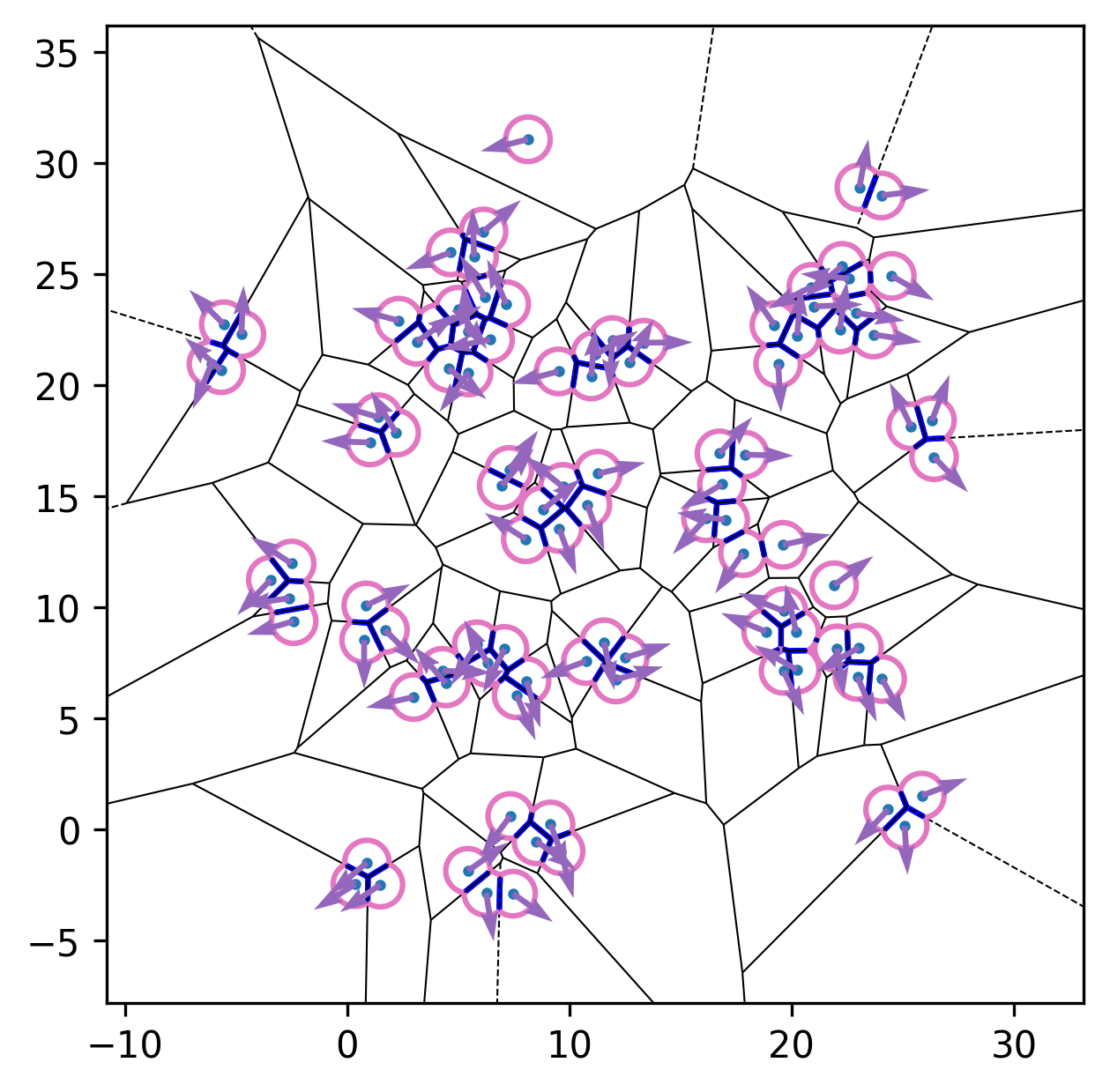
With contact truncation (default). |
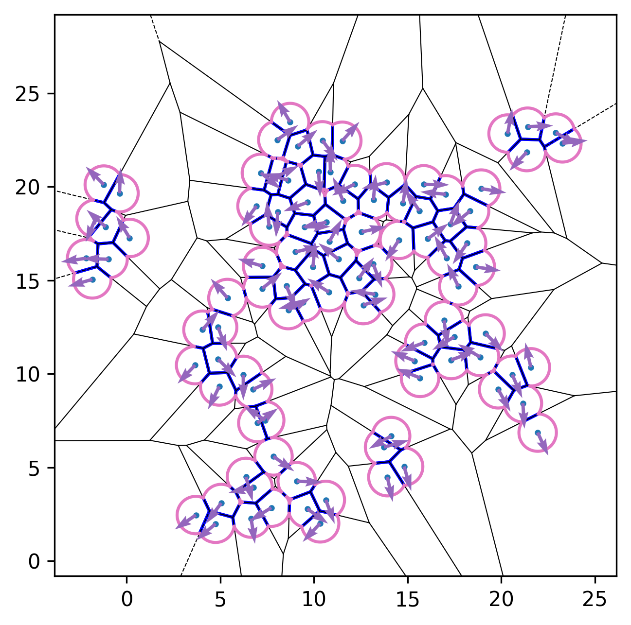
No contact truncation (\(\delta=0\)). |
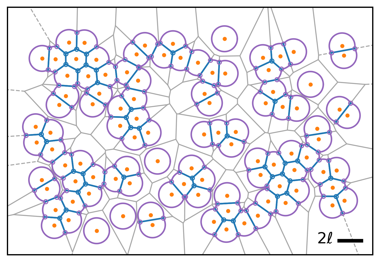
2.3. Connectivity between cells
PyAFV can directly output the cell-cell connectivity from the finite Voronoi diagram, where any two connected cells share a straight Voronoi edge.
import numpy as np
import matplotlib.pyplot as plt
from matplotlib.collections import LineCollection
import pyafv as afv


np.random.seed(42)

N = 200         # number of cells
radius = 1.0    # maximal radius

# Parameter set
phys = afv.PhysicalParams(
    r=radius,
    A0=np.pi*(radius**2),
    P0=4.8*radius,
    KA=1.0,
    KP=1.0,
    Lambda=0.2
)

# Initial positions
pts = np.random.rand(N, 2)*0.3 + 0.35  # shape (N,2)
pts *= 70.

# Initialize simulator
sim = afv.FiniteVoronoiSimulator(pts, phys)
diag = sim.build()
connect = diag["connections"]

# Plot initial configuration
fig, ax = plt.subplots()
sim.plot_2d(ax=ax)

# Plot the connections between cells
num_connections = connect.shape[0]
if num_connections > 0:
    i_masked = connect[:, 0]
    j_masked = connect[:, 1]
    # Build list of segments (line endpoints) for visualization, shape: (num_pairs, 2, 2)
    segments = np.stack([pts[i_masked], pts[j_masked]], axis=1)
    # Create LineCollection
    lc = LineCollection(segments, colors="C7", linewidths=1.5, zorder=0)
    ax.add_collection(lc)

plt.show()
2.4. Custom plotting
See examples/jupyter/custom_plot.ipynb for an example of custom plotting using PyAFV, or you can run the notebook directly on Google Colab by clicking the badge above.
This example, together with the example in the section using periodic boundary conditions, show how to use pyafv.FiniteVoronoiSimulator.build() returned dict to plot the Voronoi diagram with custom styling, including coloring cells by their area and customizing edge colors and widths. Both a serial version (for illustration) and a vectorized version (⚡much faster) of the custom plotting routine are provided in the notebooks.
Important
Starting from v0.4.10, we also provide a standalone utility function pyafv.visualize_2d(), which wraps the vectorized plotting routine for easier reuse (see the next section). This function is generally preferred over the original pyafv.FiniteVoronoiSimulator.plot_2d() method.
This notebook also shows how to access additional internal information via pyafv.FiniteVoronoiSimulator._build_voronoi_with_extensions() and pyafv.FiniteVoronoiSimulator._per_cell_geometry() for advanced plotting. The public pyafv.FiniteVoronoiSimulator.build() method serves as a higher-level wrapper around these two and other lower-level routines.
- FiniteVoronoiSimulator._build_voronoi_with_extensions(joggle=False)[source]
Build standard Voronoi structure for current points.
For N<=2, emulate regions. For N>=3, extend infinite ridges, add extension vertices, and update regions accordingly. Return the augmented structures.
Warning
This is an internal method. Use with caution.
- Parameters:
joggle (bool) – Whether to joggle input points (N>=3) slightly to avoid precision issues (e.g., collinearities, co-circularities).
- Returns:
A tuple containing:
vor: SciPy Voronoi object for current points with extensions.
vertices_all: (M,2) array of all Voronoi vertices including extensions.
ridge_vertices_all: (R,2) array of vertex indices for each ridge, including extensions.
num_vertices: Number of Voronoi vertices before adding extension.
vertexpair2ridge: dict mapping vertex index pairs to ridge index.
vertex_points: dict mapping vertex index to list of associated point indices.
- Return type:
tuple[Voronoi, ndarray, ndarray, int, dict[tuple[int,int], int], dict[int, list[int]]]
- FiniteVoronoiSimulator._per_cell_geometry(vor, vertices_all, ridge_vertices_all, num_vertices, vertexpair2ridge)[source]
Build the finite Voronoi per-cell geometry and energy contributions.
- Iterate each cell to:
sort polygon/arc vertices around each cell
classify edges (1 = straight Voronoi edge; 0 = circular arc)
compute area/perimeter for each cell
accumulate derivatives w.r.t. vertices (dA_poly/dh, dP_poly/dh)
register “outer” vertices created at arc intersections and track their point pairs
Warning
This is an internal method. Use with caution.
- Parameters:
vor (Voronoi) – SciPy Voronoi object for current points with extensions.
vertices_all (ndarray) – (M,2) array of all Voronoi vertices including extensions.
ridge_vertices_all (ndarray) – (R,2) array of vertex indices for each ridge.
num_vertices (int) – Number of Voronoi vertices before adding extension.
vertexpair2ridge (dict[tuple[int, int], int]) – dict mapping vertex index pairs to ridge index.
- Returns:
A diagnostics dictionary containing:
vertex_in_id: set of inner vertex ids.
vertex_out_id: set of outer vertex ids.
vertices_out: (L,2) array of outer vertex coordinates.
vertex_out_points: (L,2) array of point index pairs associated with each outer vertex.
vertex_out_da_dtheta: Array of dA/dtheta for all outer vertices.
vertex_out_dl_dtheta: Array of dL/dtheta for all outer vertices.
dA_poly_dh: Array of dA_polygon/dh for each vertex.
dP_poly_dh: Array of dP_polygon/dh for each vertex.
area_list: Array of polygon areas for each cell.
perimeter_list: Array of polygon perimeters for each cell.
arclen_list: Array of non-contacting arc lengths for each cell.
point_edges_type: List of lists of edge types per cell.
point_vertices_f_idx: List of lists of vertex ids per cell.
num_vertices_ext: Number of vertices including infinite extension vertices.
coord_nums: (N,) integer array of coordination numbers per cell.
- Return type:
2.4.1. A standalone plotting utility
Inspired by the custom plotting examples used in daily research, we have implemented a standalone plotting utility pyafv.visualize_2d() that can be used to plot the finite Voronoi diagram with color-filled cells and customizable styling. A simple example usage is shown below:
import numpy as np
import matplotlib.pyplot as plt
import pyafv as afv

N = 100                                          # number of cells
pts = np.random.rand(N, 2) * 10                  # initial positions
params = afv.PhysicalParams(r=1.0)               # use default parameter values
sim = afv.FiniteVoronoiSimulator(pts, params)    # initialize the simulator
diag = sim.build()                               # compute forces and geometry

fig, ax = plt.subplots()
afv.visualize_2d(pts, diag, r=1.0, ax=ax)        # visualize the FV diagram
plt.show()
This pyafv.visualize_2d() function is designed to be flexible and efficient (vectorized), and it should satisfy most common plotting needs for 2D finite Voronoi diagrams.
- visualize_2d(pts, diag, r, ax=None, *, selected=None, **kw)[source]
Visualize a 2D snapshot using the diagnostic dictionary diag generated by
pyafv.FiniteVoronoiSimulator.build(). This is basically a wrapper around the vectorized custom plotting functions from the example notebooks and generally preferred over the originalpyafv.FiniteVoronoiSimulator.plot_2d()method. The plotting style followsscipy.spatial.voronoi_plot_2d().Note
If you are visualizing a diag from
ParallelFiniteVoronoiSimulator.build(), you should usevisualize_2d_parallel()instead.- Parameters:
pts (ndarray) – An (N, 2) array of point coordinates.
diag (dict[str, object]) – A diagnostic dict containing Voronoi diagram information.
r (float) – Maximum radius (or denoted as \(\ell\)) used for drawing arcs.
ax (Axes | None) – If provided, draw into the axes; otherwise create a new one.
selected (array-like | None, optional) – Cells to draw. This can be either a one-dimensional array of integer indices or a boolean mask with length equal to
len(pts). If None, draw all cells.cell_colors (color or list, optional) – A single color or a sequence of colors for filling cells, default ‘C2’. Use None for no fill. If selected is provided, full-length per-cell color sequences are sliced to the selected cells.
fill_alpha (float, optional) – Specifies the alpha for cell fills, default 0.1.
fill_zorder (float, optional) – Specifies the z-order for cell fills, default 0.
show_points (bool, optional) – Add cell center points to the plot, default False.
point_size (float, optional) – Specifies the marker area for the points, default 4. If selected is provided, full-length per-cell sequences are sliced to the selected cells.
point_colors (color or list, optional) – A single color or a sequence of colors for the points, default ‘C0’. If selected is provided, full-length per-cell color sequences are sliced to the selected cells.
point_zorder (float, optional) – Specifies the z-order for the points, default 3.
straight_colors (color | None, optional) – Color for straight contact edges, default ‘C0’. Use None to skip drawing straight edges.
straight_lw (float, optional) – Line width for straight edges, default 1.0.
straight_alpha (float, optional) – Alpha for straight edges, default 1.0.
straight_capstyle (str, optional) – Cap style for straight edges, default ‘butt’.
straight_zorder (float, optional) – Z-order for straight edges, default 2.
arc_colors (color | None, optional) – Color for arc non-contact edges, default ‘C2’. Use None to skip drawing arc edges.
arc_lw (float, optional) – Line width for arc edges, default 1.0.
arc_alpha (float, optional) – Alpha for arc edges, default 1.0.
arc_capstyle (str, optional) – Cap style for arc edges, default ‘butt’.
arc_zorder (float, optional) – Z-order for arc edges, default 1.
auto_adjust_bounds (bool, optional) – Whether to automatically adjust the plot bounds to fit the diagram, default True.
- Returns:
The matplotlib figure object representing the entire canvas.
- Return type:
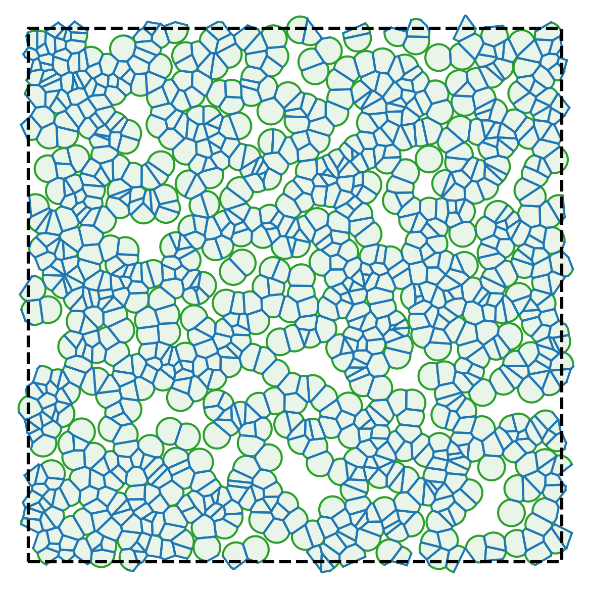
2.5. Periodic boundary conditions
PyAFV uses open boundary conditions in 2D by default, but it is also possible to implement periodic boundary conditions via a tiling of the edge regions. See examples/jupyter/periodic_plotting.ipynb for an example (or you can run the notebook directly on Google Colab by clicking the badge above), and the generated figure is shown below:
Note
Starting from v0.4.10, the tiling routine is also wrapped as a utility function pyafv.tile_pbc() (experimental).
2.6. Varying cell target areas from cell to cell
Starting from PyAFV v0.3.5, the simulator supports cell-specific preferred areas, allowing the target area \(A_0\) to vary from cell to cell, i.e., \(\{A_{0,i}\}\) .
A new read-only property pyafv.FiniteVoronoiSimulator.preferred_areas has been added. It returns the current preferred areas for all cells:
- FiniteVoronoiSimulator.preferred_areas
Preferred areas \(\{A_{0,i}\}\) for all cells (read-only).
- Returns:
A copy of the internal preferred area array.
- Return type:
To modify the preferred areas, the method pyafv.FiniteVoronoiSimulator.update_preferred_areas() is provided:
- FiniteVoronoiSimulator.update_preferred_areas(A0)[source]
Update the preferred areas for all cells.
- Parameters:
A0 (float | ndarray) – New preferred area(s) for all cells, either as a scalar or as an array of shape (N,).
- Raises:
ValueError – If A0 does not match cell number.
- Return type:
None
Here is an example usage:
import numpy as np
from pyafv import FiniteVoronoiSimulator, PhysicalParams

# Initialize simulator
N = 100
pts = np.random.rand(N, 2) * 10
phys = PhysicalParams(r=1.0, A0=np.pi)
sim = FiniteVoronoiSimulator(pts, phys)

# Set varying preferred areas per cell
varying_A0 = np.pi + 0.2 * np.random.randn(N)
sim.update_preferred_areas(varying_A0)

# Access via property
print(sim.preferred_areas)  # shape: (N,)

# Run simulation...
In addition, the pyafv.FiniteVoronoiSimulator.update_positions() method now accepts an optional second argument to update the preferred areas:
- FiniteVoronoiSimulator.update_positions(pts, A0=None)[source]
Update cell center positions.
Note
If the number of cells changes, the preferred areas for all cells are reset to the default value—defined either at simulator instantiation or by
update_params()—unless A0 is explicitly specified.- Parameters:
- Raises:
ValueError – If pts does not have shape (N,2).
ValueError – If A0 is an array and does not have shape (N,).
- Return type:
None
And the pyafv.FiniteVoronoiSimulator.update_params() method will also re-initialize the preferred areas for all cells using the supplied value of A0 in phys:
- FiniteVoronoiSimulator.update_params(phys)[source]
Update physical parameters.
- Parameters:
phys (PhysicalParams) – New
PhysicalParamsobject.- Raises:
TypeError – If phys is not an instance of
PhysicalParams.- Return type:
None
Warning
This also resets all preferred cell areas to the new value of A0.