4. Performance

4.1. Measuring performance

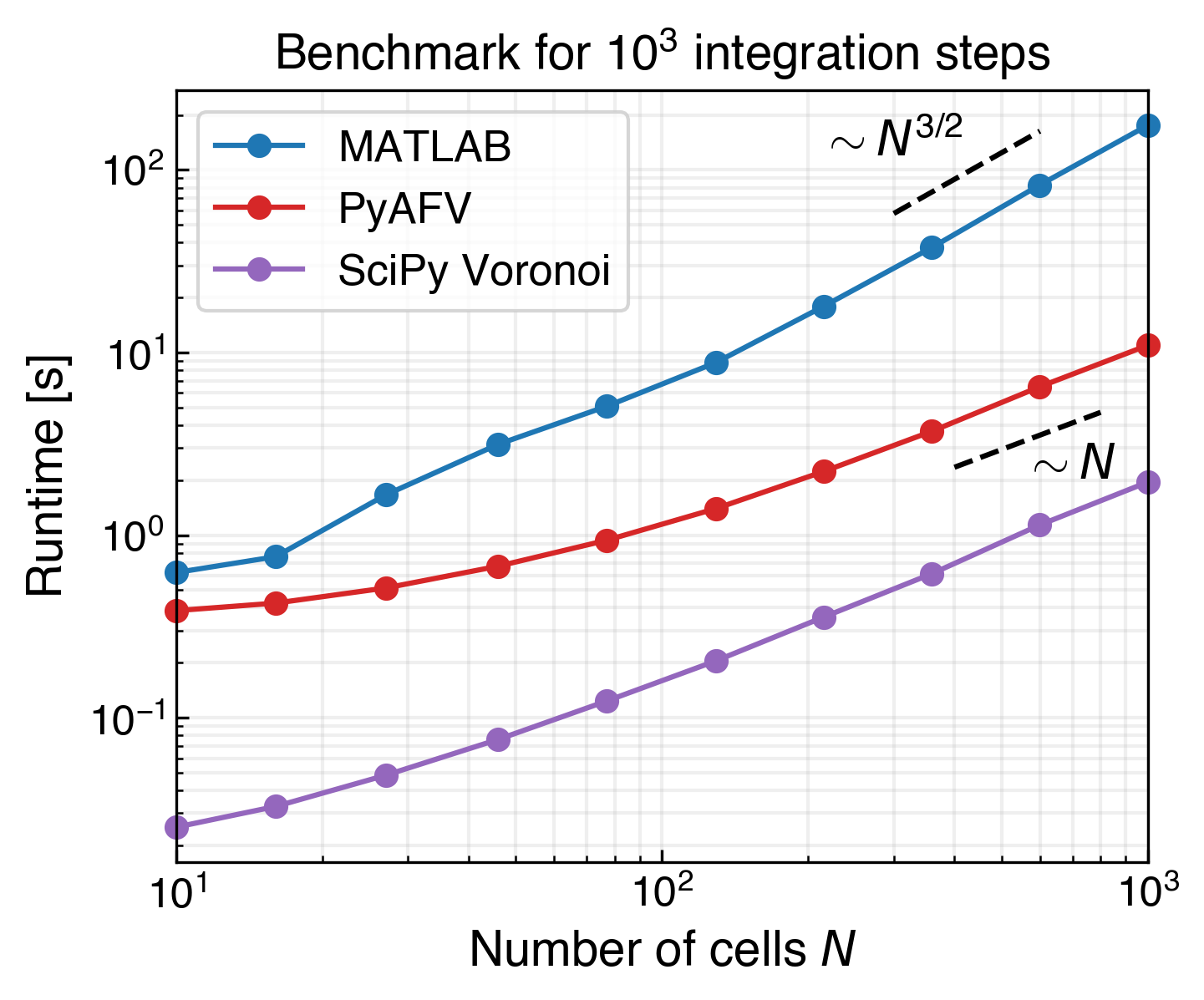
PyAFV has been benchmarked against the MATLAB implementation of the active finite Voronoi model from Ref. [1] by measuring the wall-clock runtime for simulations of varying system sizes. The results are shown in the figure; each data point corresponds to \(10^3\) integration steps, averaged over three independent runs. The results show that PyAFV exhibits near-linear scaling, approximately \(\mathcal{O}(N)\)—comparable to the scaling behavior of SciPy’s Voronoi implementation scipy.spatial.Voronoi—whereas the original MATLAB code scales more steeply, at roughly \(\mathcal{O}(N^{3/2})\). This difference will lead to a significant speedup, particularly for large systems (\(N\gtrsim 10^3\)).

Note

All benchmark results were obtained on a MacBook Pro (14-in, 2024) equipped with an Apple M4 Pro chip (12-core) and 24 GB of RAM, running macOS 15.6. The MATLAB implementation was executed using MATLAB R2025a, while PyAFV was run using Python 3.13.5 with the PyAFV v0.4.3 default Cython backend (PyAFV v0.4.12 for parallel build benchmark).

4.2. Benchmarking backends

In addition, there is a set of lightweight benchmarks in tests using pytest-benchmark, e.g., test_bench_build.py compares the runtimes of the Cython and pure-Python backends . To run it:

(.venv) $ uv run pytest tests/test_bench_build.py --benchmark-only --benchmark-warmup on --benchmark-histogram

This will display the benchmark results and generate an interactive SVG histogram file (click to see the detailed timing results for each method):

The histogram above summarizes the runtimes of the core routines invoked by pyafv.FiniteVoronoiSimulator.build() for a system of \(N=1000\) cells. The test_scipy_voronoi benchmark measures the execution time of SciPy’s Voronoi tessellation, which serves as a baseline for comparison. This SciPy routine is called internally by pyafv.FiniteVoronoiSimulator._build_voronoi_with_extensions(), corresponding to the test_build_voronoi benchmark shown in the histogram. From this comparison, we see that SciPy’s Voronoi computation accounts for approximately 60% of the total runtime of that method.

Hint

The suffixes [accel] and [fallback] in the benchmark names indicate whether the Cython backend or the pure-Python fallback implementation was used.

The remaining dominant cost arises from the additional per-cell processing performed in pyafv.FiniteVoronoiSimulator._per_cell_geometry(). As shown in the histogram, the Cython-backed implementation substantially reduces the runtime of this step, bringing it down to a level comparable to that of SciPy’s Voronoi tessellation.

4.3. Benchmarking parallel build

Parallel build-time benchmark — Build-time benchmark for `pyafv.FiniteVoronoiSimulator` and `pyafv.ParallelFiniteVoronoiSimulator`.

The figure shows the cost of a single pyafv.FiniteVoronoiSimulator.build() call with connect=False against the domain-decomposed multiprocess implementation. For each system size, the same ten randomly generated point sets were used for all methods; the bars show the mean build time, while the right panel shows the speedup relative to pyafv.FiniteVoronoiSimulator. Parallel timings were measured with a persistent worker pool and three unmeasured warm-up builds, so the reported times do not include one-time worker startup.

For very small systems, multiprocessing overhead dominates. In this benchmark, the parallel implementation is slower than the single-process simulator at \(N=100\), but becomes faster by \(N=1000\). For larger systems, local domain decomposition gives substantial speedups: the 4 x 3 setup reaches about \(4.9\times\) at \(N=10^4\), \(6.8\times\) at \(N=10^5\), and \(6.9\times\) at \(N=10^6\). The speedup is not perfectly linear in the number of workers, likely because the benchmark was run on a laptop with 8 performance cores and 4 efficiency cores rather than on a uniform multi-core CPU.

The optimal decomposition depends on the number of points and the CPU resources available on the machine. In this benchmark, using more domains generally helps over the tested range, but this tradeoff depends on halo overhead and should be checked for each workload.