1. Getting started
1.1. Installation
PyAFV supports Python ≥ 3.10, < 3.15, and has been tested on major operating systems including Linux, macOS, and Windows, for both x86-64 and ARM64 architectures.
Note
Python 3.14t, the free-threaded build that runs without the Global Interpreter Lock (GIL), is also supported starting with PyAFV v0.3.8.
Python 3.10 on Windows ARM64 (not x86-64) is the only untested configuration. The build succeeds and the wheel is available on PyPI, but automated testing is unavailable due to the absence of a supported GitHub Actions runner for this configuration.
1.1.1. Install using pip


The package is available on PyPI, so you should be able to install it using pip directly:
(.venv) $ pip install pyafv
After installation, verify that it was successful by importing the package in Python and checking the version:
>>> import pyafv
>>> pyafv.__version__
'0.3.9'
Note
On HPC clusters, global Python path can contaminate the runtime environment. You may need to clear it explicitly using unset PYTHONPATH or prefixing the pip command with PYTHONPATH="".
1.1.2. Install from source
Installing from source can be necessary if pip installation does not work. First, download the source code of pyafv from GitHub or PyPI.
1.1.2.1. Required prerequisites
The required packages are listed in the table below:
Package |
Minimum Version |
Usage |
|---|---|---|
numpy |
1.26.4 |
Numerical computations |
scipy |
1.13.1 |
Scientific computations |
matplotlib |
3.8.4 |
Plotting and visualization |
Unzip the downloaded source code and navigate to the root directory of the package. Then, run the following command to install:
(.venv) $ pip install .
Note
A C/C++ compiler is required if you are building from source, since some components of PyAFV are implemented in Cython for performance optimization.
1.1.2.2. Windows MinGW GCC
If you are using MinGW GCC (rather than MSVC) on Windows, to build from the source code, add a setup.cfg at the repository root before running pip install . with the following content:
# setup.cfg
[build_ext]
compiler=mingw32
1.2. A simple example
Now that you have installed PyAFV, here is a simple example to get you started. Begin by importing the required libraries and generating 100 random points in two dimensions:
import numpy as np
import pyafv

N = 100                                           # number of cells
pts = np.random.rand(N, 2) * 10                   # initial positions
Next, create a pyafv.PhysicalParams object to specify the physical parameters of the simulation:
params = pyafv.PhysicalParams(r=1.0) # use default parameter values
- class pyafv.PhysicalParams(r=1.0, A0=3.141592653589793, P0=4.8, KA=1.0, KP=1.0, lambda_tension=0.2, delta=0.0)[source]
Physical parameters for the active-finite-Voronoi (AFV) model.
- Caveat:
Frozen dataclass is used for
PhysicalParamsto ensure immutability of instances.
- Parameters:
r (float) – Radius (maximal) of the Voronoi cells.
A0 (float) – Preferred area of the Voronoi cells.
P0 (float) – Preferred perimeter of the Voronoi cells.
KA (float) – Area elasticity constant.
KP (float) – Perimeter elasticity constant.
lambda_tension (float) – Tension difference between non-contacting edges and contacting edges.
delta (float) – Small offset to avoid singularities in computations.
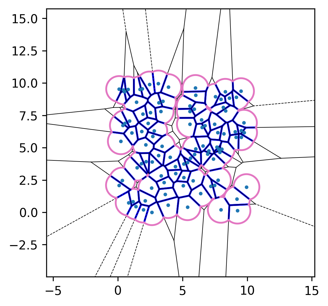
Finally, initialize the simulator by constructing a pyafv.FiniteVoronoiSimulator instance and visualize the resulting Voronoi diagram:
sim = pyafv.FiniteVoronoiSimulator(pts, params)   # initialize the simulator
sim.plot_2d(show=True)                            # visualize the Voronoi diagram
The plotting routine plot_2d() is provided by:
- FiniteVoronoiSimulator.plot_2d(ax=None, show=False)[source]
Build the finite-Voronoi structure and render a 2D snapshot.
Basically a wrapper of
_build_voronoi_with_extensions()and_per_cell_geometry()functions + plot.
To compute the conservative forces and extract detailed geometric information (e.g., cell areas, vertices, and edges), call:
sim.build() # compute forces and geometry
The returned object diag is a Python dict containing these quantities.
- FiniteVoronoiSimulator.build(connect=True)[source]
Build the finite-Voronoi structure and compute forces, returning a dictionary of diagnostics.
- Do the following:
Build Voronoi (+ extensions)
Get cell connectivity
Compute per-cell quantities and derivatives
Assemble forces
- Parameters:
connect (bool) – Whether to compute cell connectivity information. Setting this to
Falsesaves some computation time (though very marginal) when connectivity is not needed.- Returns:
A dictionary containing geometric properties with keys:
forces: (N,2) array of forces on cell centers
areas: (N,) array of cell areas
perimeters: (N,) array of cell perimeters
vertices: (M,2) array of all Voronoi + extension vertices
edges_type: List-of-lists of edge types per cell (1=straight, 0=circular arc)
regions: List-of-lists of vertex indices per cell
connections: (K,2) array of connected cell index pairs
- Return type:
For more examples and detailed usage instructions, please refer to the Examples and API reference sections.