2. Examples
Note
To run the examples below, install the tqdm package for progress bars (using pip). The Jupyter Notebooks in examples/jupyter/ additionally require jupyter and ipywidgets as well.
2.1. Relaxation to mechanical equilibrium
The following example shows how 100 cells relax to mechanical equilibrium from a squeezed initial configuration using the PyAFV package.
import numpy as np
import matplotlib.pyplot as plt
import tqdm
import pyafv as afv

np.random.seed(42)

N = 100         # number of cells
radius = 1.0    # maximal radius
mu = 1.0        # mobility
dt = 0.01       # time step

# Parameter set
phys = afv.PhysicalParams(
    r=radius,
    A0=np.pi*(radius**2),
    P0=4.8*radius,
    KA=1.0,
    KP=1.0,
    lambda_tension=0.2
)

# Initial positions
pts = np.random.rand(N, 2)*0.3 + 0.35  # shape (N,2)
pts *= 25.

# Initialize simulator
sim = afv.FiniteVoronoiSimulator(pts, phys)

# Plot initial configuration
fig, ax = plt.subplots()
sim.plot_2d(ax=ax)
plt.show()

# Relaxation to mechanical equilibrium
for _ in tqdm.tqdm(range(1000), desc="Relaxation"):
    diag = sim.build()
    forces = diag["forces"]
    pts += mu * forces * dt
    sim.update_positions(pts)

# Plot relaxed configuration
fig, ax = plt.subplots()
sim.plot_2d(ax=ax)
plt.show()
See the plotted figures below:
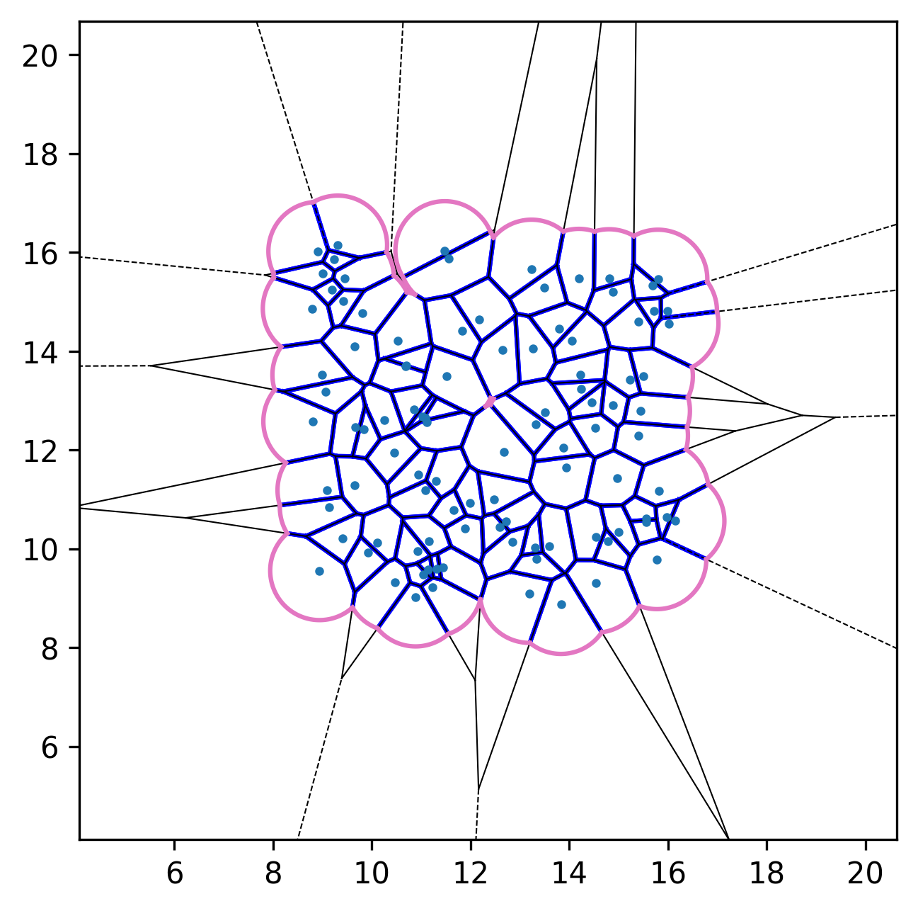
Initial configuration. |
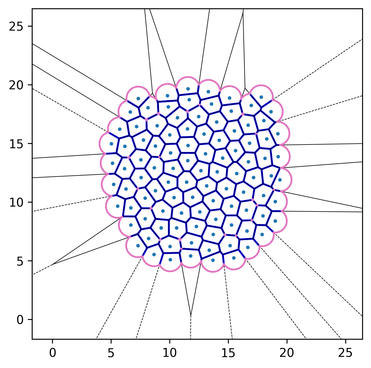
After relaxation. |
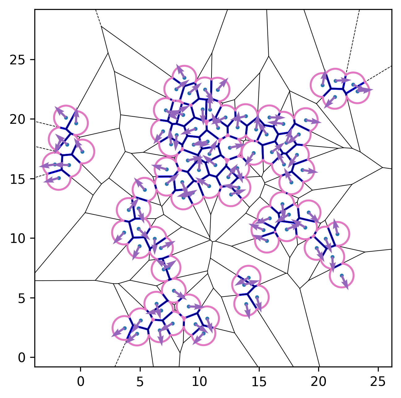
2.2. Active-Finite-Voronoi (AFV) dynamics
We can incorporate self-propulsion (active-Brownian-like dynamics) for each cell to model active-matter systems. The resulting equation of motion is
where \(\mu\) is the mobility, the interaction force on cell \(\mathbf{F}_i=-\nabla_i E\), and \(\mathbf{n}_i = (\cos \theta_i, \sin \theta_i)\) is a unit orientation vector. The orientation evolves according to
where the noise satisfies \(\langle \eta_i(t) \rangle = 0\) and \(\langle \eta_i(t)\eta_j(t') \rangle = \delta_{ij}\,\delta(t - t')\).
import numpy as np
import matplotlib.pyplot as plt
import tqdm
import pyafv as afv


np.random.seed(42)

N = 100         # number of cells
radius = 1.0    # maximal radius
mu = 1.0        # mobility
va = 2.4        # self-propulsion speed
Dr = 0.3        # rotational diffusion constant
dt = 0.01       # time step

# Parameter set
phys = afv.PhysicalParams(
    r=radius,
    A0=np.pi*(radius**2),
    P0=4.8*radius,
    KA=1.0,
    KP=1.0,
    lambda_tension=0.2
)

# Initial positions and orientations
pts = np.random.rand(N, 2)*0.3 + 0.35  # shape (N,2)
pts *= 25.
theta = 2. * np.pi * np.random.rand(N) - np.pi

# Initialize simulator
sim = afv.FiniteVoronoiSimulator(pts, phys)

# Relaxation to mechanical equilibrium
for _ in tqdm.tqdm(range(200), desc="Relaxation"):
    diag = sim.build()
    pts += mu * diag["forces"] * dt
    sim.update_positions(pts)

# Active dynamics
for _ in tqdm.tqdm(range(1000), desc="Active dynamics"):
    diag = sim.build()
    forces = diag["forces"]

    active_velocity = va * np.column_stack((np.cos(theta), np.sin(theta)))

    pts += (mu * forces + active_velocity) * dt

    # Gaussian white noise
    theta += np.sqrt(2 * Dr * dt) * np.random.randn(N)

    sim.update_positions(pts)


fig, ax = plt.subplots()
sim.plot_2d(ax=ax)
# Plot cell orientations
ax.quiver(pts[:, 0], pts[:, 1], np.cos(theta),
          np.sin(theta), color='C4', scale=20, zorder=3)
plt.show()
See the plotted figure below:
2.3. Connectivity between cells
PyAFV can directly output the cell-cell connectivity from the finite Voronoi diagram, where any two connected cells share a straight Voronoi edge.
import numpy as np
import matplotlib.pyplot as plt
from matplotlib.collections import LineCollection
import pyafv as afv


np.random.seed(42)

N = 200         # number of cells
radius = 1.0    # maximal radius

# Parameter set
phys = afv.PhysicalParams(
    r=radius,
    A0=np.pi*(radius**2),
    P0=4.8*radius,
    KA=1.0,
    KP=1.0,
    lambda_tension=0.2
)

# Initial positions
pts = np.random.rand(N, 2)*0.3 + 0.35  # shape (N,2)
pts *= 70.

# Initialize simulator
sim = afv.FiniteVoronoiSimulator(pts, phys)
diag = sim.build()
connect = diag["connections"]

# Plot initial configuration
fig, ax = plt.subplots()
sim.plot_2d(ax=ax)

# Plot the connections between cells
num_connections = connect.shape[0]
if num_connections > 0:
    i_masked = connect[:, 0]
    j_masked = connect[:, 1]
    # Build list of segments (line endpoints) for visualization, shape: (num_pairs, 2, 2)
    segments = np.stack([pts[i_masked], pts[j_masked]], axis=1)
    # Create LineCollection
    lc = LineCollection(segments, colors="C7", linewidths=1.5, zorder=0)
    ax.add_collection(lc)

plt.show()
2.4. Custom plotting
See examples/jupyter/custom_plot.ipynb for an example of custom plotting using PyAFV.
This example shows how to use pyafv.FiniteVoronoiSimulator.build() returned dict to plot the Voronoi diagram with custom styling, including coloring cells by their area and customizing edge colors and widths.
- FiniteVoronoiSimulator.build()
Build the finite-Voronoi structure and compute forces, returning a dictionary of diagnostics.
- Do the following:
Build Voronoi (+ extensions)
Get cell connectivity
Compute per-cell quantities and derivatives
Assemble forces
- Returns:
A dictionary containing geometric properties with keys:
forces: (N,2) array of forces on cell centers
areas: (N,) array of cell areas
perimeters: (N,) array of cell perimeters
vertices: (M,2) array of all Voronoi + extension vertices
edges_type: list-of-lists of edge types per cell (1=straight, 0=circular arc)
regions: list-of-lists of vertex indices per cell
connections: (M’,2) array of connected cell index pairs
- Return type:
This example also shows how to access additional internal information via pyafv.FiniteVoronoiSimulator._build_voronoi_with_extensions() and pyafv.FiniteVoronoiSimulator._per_cell_geometry() for advanced plotting. The public build() method serves as a higher-level wrapper around these two and other lower-level routines.
- FiniteVoronoiSimulator._build_voronoi_with_extensions()
Build standard Voronoi structure for current points.
For N<=2, emulate regions. For N>=3, extend infinite ridges, add extension vertices, and update regions accordingly. Return the augmented structures.
Warning
This is an internal method. Use with caution.
- Returns:
A tuple containing:
vor: SciPy Voronoi object for current points with extensions.
vertices_all: (M,2) array of all Voronoi vertices including extensions.
ridge_vertices_all: list of lists of vertex indices for each ridge, including extensions.
num_vertices: Number of Voronoi vertices before adding extension.
vertexpair2ridge: dict mapping vertex index pairs to ridge index.
vertex_points: dict mapping vertex index to list of associated point indices.
- Return type:
tuple[scipy.spatial.Voronoi, numpy.ndarray, list[list[int]], int, dict[tuple[int,int], int], dict[int, list[int]]]
- FiniteVoronoiSimulator._per_cell_geometry(vor, vertices_all, ridge_vertices_all, num_vertices, vertexpair2ridge)
Build the finite-Voronoi per-cell geometry and energy contributions.
- Iterate each cell to:
sort polygon/arc vertices around each cell
classify edges (1 = straight Voronoi edge; 0 = circular arc)
compute area/perimeter for each cell
accumulate derivatives w.r.t. vertices (dA_poly/dh, dP_poly/dh)
register “outer” vertices created at arc intersections and track their point pairs
Warning
This is an internal method. Use with caution.
- Parameters:
vor (Voronoi) – SciPy Voronoi object for current points with extensions.
vertices_all (ndarray) – (M,2) array of all Voronoi vertices including extensions.
ridge_vertices_all (ndarray) – list of lists of vertex indices for each ridge, including extensions.
num_vertices (int) – Number of Voronoi vertices before adding extension.
vertexpair2ridge (dict[tuple[int, int], int]) – dict mapping vertex index pairs to ridge index.
- Returns:
A diagnostics dictionary containing:
vertex_in_id: set of inner vertex ids.
vertex_out_id: set of outer vertex ids.
vertices_out: (L,2) array of outer vertex coordinates.
vertex_out_points: (L,2) array of point index pairs associated with each outer vertex.
vertex_out_da_dtheta: array of dA/dtheta for all outer vertices.
vertex_out_dl_dtheta: array of dL/dtheta for all outer vertices.
dA_poly_dh: array of dA_polygon/dh for each vertex.
dP_poly_dh: array of dP_polygon/dh for each vertex.
area_list: array of polygon areas for each cell.
perimeter_list: array of polygon perimeters for each cell.
point_edges_type: list of lists of edge types per cell.
point_vertices_f_idx: list of lists of vertex ids per cell.
num_vertices_ext: number of vertices including infinite extension vertices.
- Return type:
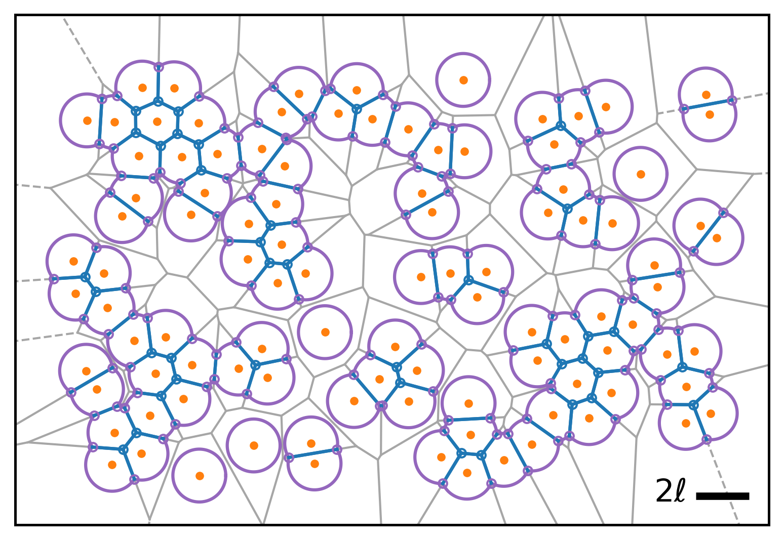
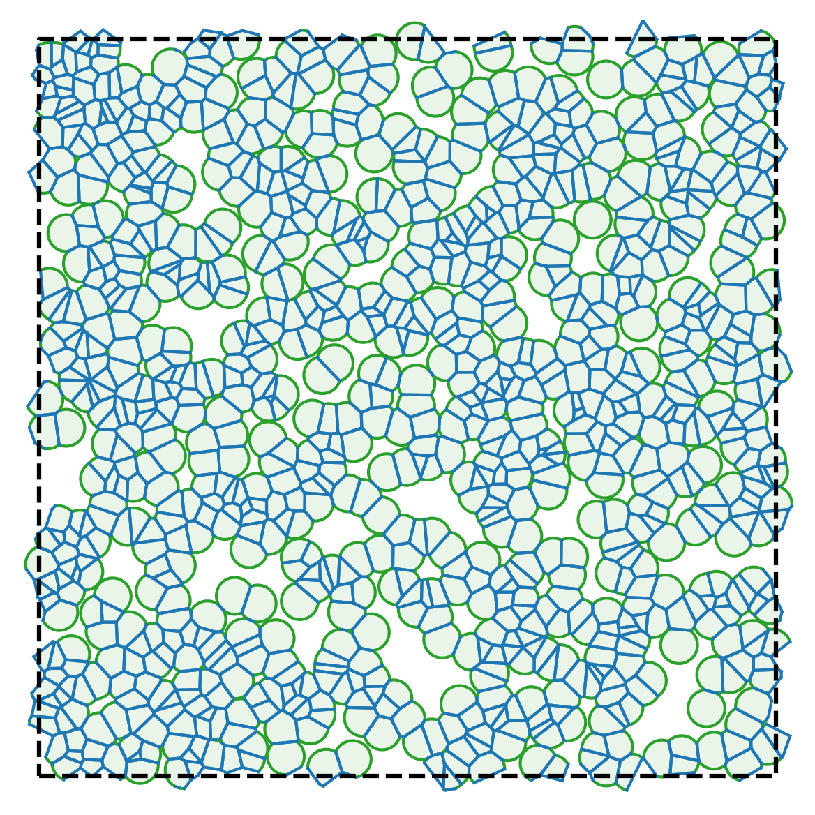
2.5. Periodic boundary conditions
PyAFV uses open boundary conditions in 2D by default, but it is also possible to implement periodic boundary conditions via a tiling of the edge regions. See examples/jupyter/periodic_plotting.ipynb for an example, and the generated figure is shown below:
2.6. Varying cell target areas from cell to cell
Starting from PyAFV v0.3.5, the simulator supports cell-specific preferred areas, allowing the target area \(A_0\) to vary from cell to cell.
A new read-only property pyafv.FiniteVoronoiSimulator.preferred_areas has been added. It returns the current preferred areas of all cells:
- FiniteVoronoiSimulator.preferred_areas
Preferred areas for all cells (read-only).
- Returns:
A copy of the internal preferred area array.
- Return type:
To modify the preferred areas, the method pyafv.FiniteVoronoiSimulator.update_preferred_areas() is provided:
- FiniteVoronoiSimulator.update_preferred_areas(A0)
Update the preferred areas for all cells.
- Parameters:
- Raises:
ValueError – If A0 does not match cell number.
- Return type:
None
Here is an example usage:
import numpy as np
from pyafv import FiniteVoronoiSimulator, PhysicalParams

# Initialize simulator
N = 100
pts = np.random.rand(N, 2) * 10
phys = PhysicalParams(r=1.0, A0=np.pi)
sim = FiniteVoronoiSimulator(pts, phys)

# Set varying preferred areas per cell
varying_A0 = np.pi + 0.2 * np.random.randn(N)
sim.update_preferred_areas(varying_A0)

# Access via property
print(sim.preferred_areas)  # shape: (N,)

# Run simulation...
In addition, the pyafv.FiniteVoronoiSimulator.update_positions() method now accepts an optional second argument to update the preferred areas:
- FiniteVoronoiSimulator.update_positions(pts, A0=None)
Update cell center positions.
Note
If the number of points changes, the preferred areas for all cells are reset to the default value (set when initializing the simulator instance or by
update_params()) unless specified via the A0 argument.- Parameters:
- Raises:
ValueError – If pts does not have shape (N,2).
ValueError – If A0 is an array and does not have shape (N,).
- Return type:
None
And the pyafv.FiniteVoronoiSimulator.update_params() method will also re-initialize the preferred areas for all cells using the supplied value of A0 in phys:
- FiniteVoronoiSimulator.update_params(phys)
Update physical parameters.
- Parameters:
phys (PhysicalParams) – New PhysicalParams object.
- Raises:
TypeError – If phys is not an instance of PhysicalParams.
- Return type:
None
Warning
This also resets all preferred cell areas to the new value of A0.